Cluster Speed Benchmarks
NER (BiLSTM-CNN-Char Architecture) Benchmark Experiment
- Dataset: 1000 Clinical Texts from MTSamples Oncology Dataset, approx. 500 tokens per text.
- Driver : Standard_D4s_v3 - 16 GB Memory - 4 Cores
- Enable Autoscaling : False
- Cluster Mode : Standart
- Worker :
- Standard_D4s_v3 - 16 GB Memory - 4 Cores
- Standard_D4s_v2 - 28 GB Memory - 8 Cores
- Versions:
- Databricks Runtime Version : 8.3(Scala 2.12, Spark 3.1.1)
- spark-nlp Version: v5.4.1
- spark-nlp-jsl Version : v5.4.1
- Spark Version : v5.4.1
- Spark NLP Pipeline:
# NER Pipelime
nlpPipeline = Pipeline(stages=[
      documentAssembler,
      sentenceDetector,
      tokenizer,
      embeddings_clinical,
      clinical_ner,
      ner_converter
      ])

# Multi (2) NER Pipeline
nlpPipeline = Pipeline(stages=[
      documentAssembler,
      sentenceDetector,
      tokenizer,
      embeddings_clinical,
      clinical_ner,
      ner_converter,
      clinical_ner,
      ner_converter,
      ])

# Multi (4) NER Pipeline
nlpPipeline = Pipeline(stages=[
      documentAssembler,
      sentenceDetector,
      tokenizer,
      embeddings_clinical,
      clinical_ner,
      ner_converter,
      clinical_ner,
      ner_converter,
      clinical_ner,
      ner_converter,
      clinical_ner,
      ner_converter
      ])

# NER & RE Pipeline
nlpPipeline = Pipeline(stages=[
      documentAssembler,
      sentenceDetector,
      tokenizer,
      embeddings_clinical,
      clinical_ner,
      ner_converter,
      pos_tagger,
      dependency_parser,
      re_model
      ])
NOTES:
-
The first experiment with 5 different cluster configurations :
ner_chunkas a column in Spark NLP Pipeline (ner_converter) output data frame, exploded (lazy evaluation) asner_chunkandner_label. Then results were written as parquet and delta formats. -
A second experiment with 2 different cluster configuration : Spark NLP Pipeline output data frame (except
word_embeddingscolumn) was written as parquet and delta formats. -
In the first experiment with the most basic driver node and worker (1 worker x 4 cores) configuration selection, it took 4.64 mins and 4.53 mins to write 4 partitioned data as parquet and delta formats respectively.
-
With basic driver node and 8 workers (x8 cores) configuration selection, it took 40 seconds and 22 seconds to write 1000 partitioned data as parquet and delta formats respectively.
-
In the second experiment with basic driver node and 4 workers (x 4 cores) configuration selection, it took 1.41 mins as parquet and 1.42 mins as delta format to write 16 partitioned (exploded results) data. Without explode it took 1.08 mins as parquet and 1.12 mins as delta format to write the data frame.
-
Since given computation durations are highly dependent on different parameters including driver node and worker node configurations as well as partitions, results show that explode method increases duration %10-30 on chosen configurations.
NER Benchmark Tables
- 4 Cores setup:
- Driver: Standard_D4s_v3, 4 core, 16 GB memory
- Worker: Standard_D4s_v3, 4 core, 16 GB memory, total worker number: 1
- Input Data Count: 1000
| action | partition | NER timing |
2_NER timing |
4_NER timing |
NER+RE timing |
|---|---|---|---|---|---|
| write_parquet | 4 | 4 min 47 sec | 8 min 37 sec | 19 min 34 sec | 7 min 20 sec |
| write_deltalake | 4 | 4 min 36 sec | 8 min 50 sec | 20 min 54 sec | 7 min 49 sec |
| write_parquet | 8 | 4 min 14 sec | 8 min 32 sec | 19 min 43 sec | 7 min 27 sec |
| write_deltalake | 8 | 4 min 45 sec | 8 min 31 sec | 20 min 42 sec | 7 min 54 sec |
| write_parquet | 16 | 4 min 20 sec | 8 min 31 sec | 19 min 13 sec | 7 min 24 sec |
| write_deltalake | 16 | 4 min 45 sec | 8 min 56 sec | 19 min 53 sec | 7 min 35 sec |
| write_parquet | 32 | 4 min 26 sec | 8 min 16 sec | 19 min 39 sec | 7 min 22 sec |
| write_deltalake | 32 | 4 min 37 sec | 8 min 32 sec | 20 min 11 sec | 7 min 35 sec |
| write_parquet | 64 | 4 min 25 sec | 8 min 19 sec | 18 min 57 sec | 7 min 37 sec |
| write_deltalake | 64 | 4 min 45 sec | 8 min 43 sec | 19 min 26 sec | 7 min 46 sec |
| write_parquet | 100 | 4 min 37 sec | 8 min 40 sec | 19 min 22 sec | 7 min 50 sec |
| write_deltalake | 100 | 4 min 48 sec | 8 min 57 sec | 20 min 1 sec | 7 min 53 sec |
| write_parquet | 1000 | 5 min 32 sec | 9 min 49 sec | 22 min 41 sec | 8 min 46 sec |
| write_deltalake | 1000 | 5 min 38 sec | 9 min 55 sec | 22 min 32 sec | 8 min 42 sec |
- 8 Cores setup:
- Driver: Standard_D4s_v3, 4 core, 16 GB memory
- Worker: Standard_D4s_v3, 4 core, 16 GB memory, total worker number: 2
- Input Data Count: 1000
| action | partition | NER timing |
2_NER timing |
4_NER timing |
NER+RE timing |
|---|---|---|---|---|---|
| write_parquet | 4 | 3 min 28 sec | 6 min 9 sec | 13 min 46 sec | 5 min 32 sec |
| write_deltalake | 4 | 3 min 19 sec | 6 min 18 sec | 14 min 12 sec | 5 min 34 sec |
| write_parquet | 8 | 2 min 58 sec | 4 min 56 sec | 11 min 31 sec | 4 min 37 sec |
| write_deltalake | 8 | 2 min 38 sec | 5 min 11 sec | 11 min 50 sec | 4 min 41 sec |
| write_parquet | 16 | 2 min 43 sec | 5 min 12 sec | 11 min 27 sec | 4 min 35 sec |
| write_deltalake | 16 | 2 min 53 sec | 5 min 5 sec | 11 min 46 sec | 4 min 41 sec |
| write_parquet | 32 | 2 min 42 sec | 4 min 55 sec | 11 min 15 sec | 4 min 25 sec |
| write_deltalake | 32 | 2 min 45 sec | 5 min 14 sec | 11 min 41 sec | 4 min 41 sec |
| write_parquet | 64 | 2 min 39 sec | 5 min 7 sec | 11 min 22 sec | 4 min 29 sec |
| write_deltalake | 64 | 2 min 45 sec | 5 min 11 sec | 11 min 31 sec | 4 min 30 sec |
| write_parquet | 100 | 2 min 41 sec | 5 min 0 sec | 11 min 26 sec | 4 min 37 sec |
| write_deltalake | 100 | 2 min 42 sec | 5 min 0 sec | 11 min 43 sec | 4 min 48 sec |
| write_parquet | 1000 | 3 min 10 sec | 5 min 36 sec | 13 min 3 sec | 5 min 10 sec |
| write_deltalake | 1000 | 3 min 20 sec | 5 min 44 sec | 12 min 55 sec | 5 min 14 sec |
- 16 Cores setup:
- Driver: Standard_D4s_v3, 4 core, 16 GB memory
- Worker: Standard_D4s_v3, 4 core, 16 GB memory, total worker number: 4
- Input Data Count: 1000
| action | partition | NER timing |
2_NER timing |
4_NER timing |
NER+RE timing |
|---|---|---|---|---|---|
| write_parquet | 4 | 3 min 13 sec | 5 min 35 sec | 12 min 8 sec | 4 min 57 sec |
| write_deltalake | 4 | 3 min 26 sec | 6 min 8 sec | 12 min 46 sec | 5 min 12 sec |
| write_parquet | 8 | 1 min 55 sec | 3 min 35 sec | 8 min 19 sec | 3 min 8 sec |
| write_deltalake | 8 | 2 min 3 sec | 4 min 9 sec | 8 min 35 sec | 3 min 15 sec |
| write_parquet | 16 | 1 min 36 sec | 3 min 11 sec | 7 min 14 sec | 2 min 35 sec |
| write_deltalake | 16 | 1 min 41 sec | 3 min 2 sec | 6 min 58 sec | 2 min 39 sec |
| write_parquet | 32 | 1 min 42 sec | 3 min 16 sec | 7 min 22 sec | 2 min 41 sec |
| write_deltalake | 32 | 1 min 42 sec | 3 min 13 sec | 7 min 14 sec | 2 min 38 sec |
| write_parquet | 64 | 1 min 24 sec | 2 min 32 sec | 5 min 57 sec | 2 min 22 sec |
| write_deltalake | 64 | 1 min 21 sec | 2 min 42 sec | 5 min 43 sec | 2 min 25 sec |
| write_parquet | 100 | 1 min 24 sec | 2 min 39 sec | 5 min 59 sec | 2 min 16 sec |
| write_deltalake | 100 | 1 min 28 sec | 2 min 56 sec | 5 min 48 sec | 2 min 43 sec |
| write_parquet | 1000 | 1 min 41 sec | 2 min 44 sec | 6 min 12 sec | 2 min 27 sec |
| write_deltalake | 1000 | 1 min 40 sec | 2 min 53 sec | 6 min 18 sec | 2 min 34 sec |
- 32 Cores setup:
- Driver: Standard_D4s_v3, 4 core, 16 GB memory
- Worker: Standard_D4s_v3, 4 core, 16 GB memory, total worker number: 8
- Input Data Count: 1000
| action | partition | NER timing |
2_NER timing |
4_NER timing |
NER+RE timing |
|---|---|---|---|---|---|
| write_parquet | 4 | 3 min 24 sec | 5 min 24 sec | 16 min 50 sec | 8 min 17 sec |
| write_deltalake | 4 | 3 min 5 sec | 4 min 15 sec | 12 min 7 sec | 4 min 45 sec |
| write_parquet | 8 | 1 min 47 sec | 2 min 57 sec | 6 min 19 sec | 2 min 42 sec |
| write_deltalake | 8 | 1 min 32 sec | 2 min 52 sec | 6 min 12 sec | 2 min 32 sec |
| write_parquet | 16 | 1 min 0 sec | 1 min 57 sec | 4 min 23 sec | 1 min 38 sec |
| write_deltalake | 16 | 1 min 4 sec | 1 min 55 sec | 4 min 18 sec | 1 min 40 sec |
| write_parquet | 32 | 49 sec | 1 min 42 sec | 3 min 32 sec | 1 min 21 sec |
| write_deltalake | 32 | 54 sec | 1 min 36 sec | 3 min 41 sec | 1 min 45 sec |
| write_parquet | 64 | 1 min 13 sec | 1 min 45 sec | 3 min 42 sec | 1 min 28 sec |
| write_deltalake | 64 | 53 sec | 1 min 30 sec | 3 min 29 sec | 1 min 39 sec |
| write_parquet | 100 | 1 min 4 sec | 1 min 27 sec | 3 min 23 sec | 1 min 23 sec |
| write_deltalake | 100 | 46 sec | 1 min 22 sec | 3 min 27 sec | 1 min 22 sec |
| write_parquet | 1000 | 54 sec | 1 min 31 sec | 3 min 18 sec | 1 min 20 sec |
| write_deltalake | 1000 | 57 sec | 1 min 30 sec | 3 min 20 sec | 1 min 20 sec |
- 64 Cores setup:
- Driver: Standard_D4s_v3, 4 core, 16 GB memory
- Worker: Standard_D4s_v2, 8 core, 28 GB memory, total worker number: 8
- Input Data Count: 1000
| action | partition | NER timing |
2_NER timing |
4_NER timing |
NER+RE timing |
|---|---|---|---|---|---|
| write_parquet | 4 | 1 min 36 sec | 3 min 1 sec | 6 min 32 sec | 3 min 12 sec |
| write_deltalake | 4 | 1 min 38 sec | 3 min 2 sec | 6 min 30 sec | 3 min 18 sec |
| write_parquet | 8 | 48 sec | 1 min 32 sec | 3 min 21 sec | 1 min 38 sec |
| write_deltalake | 8 | 51 sec | 1 min 36 sec | 3 min 26 sec | 1 min 43 sec |
| write_parquet | 16 | 28 sec | 1 min 16 sec | 2 min 2 sec | 56 sec |
| write_deltalake | 16 | 31 sec | 57 sec | 2 min 2 sec | 58 sec |
| write_parquet | 32 | 20 sec | 39 sec | 1 min 22 sec | 50 sec |
| write_deltalake | 32 | 22 sec | 41 sec | 1 min 45 sec | 35 sec |
| write_parquet | 64 | 17 sec | 31 sec | 1 min 8 sec | 27 sec |
| write_deltalake | 64 | 17 sec | 32 sec | 1 min 11 sec | 29 sec |
| write_parquet | 100 | 18 sec | 33 sec | 1 min 13 sec | 30 sec |
| write_deltalake | 100 | 20 sec | 33 sec | 1 min 32 sec | 32 sec |
| write_parquet | 1000 | 22 sec | 36 sec | 1 min 12 sec | 31 sec |
| write_deltalake | 1000 | 23 sec | 34 sec | 1 min 33 sec | 52 sec |
Clinical Bert For Token Classification Benchmark Experiment
- Dataset : 7537 Clinical Texts from PubMed Dataset
- Driver : Standard_DS3_v2 - 14GB Memory - 4 Cores
- Enable Autoscaling : True
- Cluster Mode : Standart
- Worker :
- Standard_DS3_v2 - 14GB Memory - 4 Cores
- Versions :
- Databricks Runtime Version : 10.0 (Apache Spark 3.2.0, Scala 2.12)
- spark-nlp Version: v3.4.0
- spark-nlp-jsl Version : v3.4.0
- Spark Version : v3.2.0
- Spark NLP Pipeline :
nlpPipeline = Pipeline(stages=[
        documentAssembler,
        sentenceDetector,
        tokenizer,
        ner_jsl_slim_tokenClassifier,
        ner_converter,
        finisher])
NOTES:
- In this experiment, the
bert_token_classifier_ner_jsl_slimmodel was used to measure the inference time of clinical bert for token classification models in the DataBricks environment. -
In the first experiment, the data read from the parquet file is saved as parquet after processing.
- In the second experiment, the data read from the delta table was written to the delta table after it was processed.
Bert For Token Classification Benchmark Table
| Repartition | Time | |
|---|---|---|
| Read data from parquet | 2 | 26.03 mins |
| 64 | 10.84 mins | |
| 128 | 7.53 mins | |
| 1000 | 8.93 mins | |
| Read data from delta table | 2 | 40.50 mins |
| 64 | 11.84 mins | |
| 128 | 6.79 mins | |
| 1000 | 6.92 mins |
Benchmarking ML Model Architectures (TensorFlow • ONNX • OpenVINO) Across CPU and GPU
This benchmark evaluates the performance of Spark NLP for Healthcare models across three different architectures (TensorFlow, ONNX, OpenVINO) on both CPU and GPU hardware. Key findings show ONNX consistently delivers superior performance on GPU environments, while OpenVINO excels in CPU-only scenarios for supported models.
- Datasets:
- MTSamples Dataset: 1,000 clinical texts, ~500 tokens per text
- Usage: General NER and embedding benchmarks
- Assertion Test Dataset: 7,570 labeled rows
- Usage: BertForAssertionClassification evaluation
- MTSamples Dataset: 1,000 clinical texts, ~500 tokens per text
- Versions:
- spark-nlp Version: v6.1.1
- spark-nlp-jsl Version : v6.1.0
- Spark Version : v3.5.1
- Instance Types:
- CPU Machine: Colab V6e-1, 173.0 GB RAM, 44 vCPUs
- GPU Machine: Colab A100, 83.5 GB RAM, 40.0 GB GPU VRAM, 12 vCPUs
- Models Tested:
- BertSentenceEmbeddings →
sbiobert_base_cased_mli - MedicalBertForSequenceClassification →
bert_sequence_classifier_ade - BertForAssertionClassification →
assertion_bert_classification_oncology - MedicalBertForTokenClassifier →
bert_token_classifier_ner_clinical - PretrainedZeroShotNER →
zeroshot_ner_deid_subentity_merged_medium - WordEmbeddings + MedicalNerModel →
embeddings_clinical+ner_deid_subentity_augmented - WordEmbeddings + 2 MedicalNerModel →
embeddings_clinical+ner_deid_subentity_augmented+ner_deid_generic_docwise
- BertSentenceEmbeddings →
- NOTES:
- This benchmark compares Transformer architectures and ML models across CPU and GPU environments
- Hardware Context: CPU and GPU machines differ in cores and memory; comparisons should consider these hardware variations
- Preprocessing: DocumentAssembler, SentenceDetector, and Tokenizer stages were pre-processed; reported times reflect pure model execution
- Configuration: All models executed with default settings
- Timing Methodology:
%%timeit -n 3 -r 1 model.write.mode("overwrite").format("noop").save() - Results: Numbers represent average execution times across runs
- Base Pipeline Configuration:
basePipeline = Pipeline(
    stages=[
        documentAssembler,
        sentenceDetector,
        tokenizer
    ])
CPU Benchmarking
| Model | TensorFlow | ONNX | OpenVINO |
|---|---|---|---|
| BertSentenceEmbeddings | 8 min 37 sec | 4 min 46 sec | 3 min 31 sec |
| MedicalBertForSequenceClassification | 3 min 30 sec | 2 min 47 sec | N/A |
| BertForAssertionClassification | 57 sec | 33 sec | N/A |
| MedicalBertForTokenClassifier | 3 min 29 sec | 2 min 46 sec | N/A |
| PretrainedZeroShotNER | N/A | 38 min 10 sec | N/A |
| WordEmbeddings + MedicalNerModel | 25 sec | N/A | N/A |
| WordEmbeddings + 2 MedicalNerModel | 38 sec | N/A | N/A |
GPU Benchmarking
| Model | TensorFlow | ONNX | OpenVINO |
|---|---|---|---|
| BertSentenceEmbeddings | 28 min 50 sec | 12 sec | 18 min 49 sec |
| MedicalBertForSequenceClassification | 11 min 45 sec | 28 sec | N/A |
| BertForAssertionClassification | 3 min 24 sec | 8 sec | N/A |
| MedicalBertForTokenClassifier | 11 min 47 sec | 26 sec | N/A |
| PretrainedZeroShotNER | N/A | 1 min 1 sec | N/A |
| WordEmbeddings + MedicalNerModel | 2 min 24 sec | N/A | N/A |
| WordEmbeddings + 2 MedicalNerModel | 4 min 8 sec | N/A | N/A |
Key Performance Insights
- TensorFlow Baseline: Reference performance with full model support
- Model Support: TensorFlow provides the broadest model compatibility, while ONNX and OpenVINO have selective support
- ONNX Advantage: Consistently fastest on GPU across all supported models
- OpenVINO Efficiency: Best CPU performance for BertSentenceEmbeddings
- GPU vs CPU: ONNX shows dramatic GPU acceleration (e.g., BertSentenceEmbeddings: 28min → 12sec)
- Note: Benchmark results may vary based on hardware specifications, model versions, and system configurations. These results are specific to the tested environment and should be used as a relative performance guide.
NER speed benchmarks across various Spark NLP and PySpark versions
This experiment compares the ClinicalNER runtime for different versions of PySpark and Spark NLP.
In this experiment, all reports went through the pipeline 10 times and repeated execution 5 times, so we ran each report 50 times and averaged it, %timeit -r 5 -n 10 run_model(spark, model).
- Driver: Standard Google Colab environment
- Spark NLP Pipeline:
nlpPipeline = Pipeline( stages=[ documentAssembler, sentenceDetector, tokenizer, word_embeddings, clinical_ner, ner_converter ]) - Dataset: File sizes:
- report_1: ~5.34kb
- report_2: ~8.51kb
- report_3: ~11.05kb
- report_4: ~15.67kb
- report_5: ~35.23kb
| Spark NLP 4.0.0 (PySpark 3.1.2) | Spark NLP 4.2.1 (PySpark 3.3.1) | Spark NLP 4.2.1 (PySpark 3.1.2) | Spark NLP 4.2.2 (PySpark 3.1.2) | Spark NLP 4.2.2 (PySpark 3.3.1) | Spark NLP 4.2.3 (PySpark 3.3.1) | Spark NLP 4.2.3 (PySpark 3.1.2) | |
|---|---|---|---|---|---|---|---|
| report_1 | 2.36066 | 3.33056 | 2.23723 | 2.27243 | 2.11513 | 2.19655 | 2.23915 |
| report_2 | 2.2179 | 3.31328 | 2.15578 | 2.23432 | 2.07259 | 2.07567 | 2.16776 |
| report_3 | 2.77923 | 2.6134 | 2.69023 | 2.76358 | 2.55306 | 2.4424 | 2.72496 |
| report_4 | 4.41064 | 4.07398 | 4.66656 | 4.59879 | 3.98586 | 3.92184 | 4.6145 |
| report_5 | 9.54389 | 7.79465 | 9.25499 | 9.42764 | 8.02252 | 8.11318 | 9.46555 |
Results show that the different versions can have some variance in the execution time, but the difference is not too relevant.
ChunkMapper and Sentence Entity Resolver Benchmark Experiment
-
Dataset: 100 Clinical Texts from MTSamples, approx. 705 tokens and 11 chunks per text.
- Versions:
- Databricks Runtime Version: 12.2 LTS(Scala 2.12, Spark 3.3.2)
- spark-nlp Version: v5.2.0
- spark-nlp-jsl Version: v5.2.0
- Spark Version: v3.3.2
- Spark NLP Pipelines:
ChunkMapper Pipeline:
    mapper_pipeline = Pipeline().setStages([
        document_assembler,
        sentence_detector,
        tokenizer,
        word_embeddings,
        ner_model,
        ner_converter,
        chunkerMapper])
Sentence Entity Resolver Pipeline:
    resolver_pipeline = Pipeline(
        stages = [
            document_assembler,
            sentenceDetectorDL,
            tokenizer,
            word_embeddings,
            ner_model,
            ner_converter,
            c2doc,
            sbert_embedder,
            rxnorm_resolver
      ])
ChunkMapper and Sentence Entity Resolver Pipeline:
mapper_resolver_pipeline = Pipeline(
    stages = [
        document_assembler,
        sentence_detector,
        tokenizer,
        word_embeddings,
        ner_model,
        ner_converter,
        chunkerMapper,
        cfModel,
        chunk2doc,
        sbert_embedder,
        rxnorm_resolver,
        resolverMerger
])
NOTES:
-
3 different pipelines: The first pipeline with ChunkMapper, the second with Sentence Entity Resolver, and the third pipeline with ChunkMapper and Sentence Entity Resolver together.
-
3 different configurations: Driver and worker types were kept as same in all cluster configurations. Number of workers were increased gradually and set as 2, 4, 8 for DataBricks. We choosed 3 different configurations for AWS EC2 machines that have same core with DataBricks.
-
NER models were kept as same in all pipelines: Pretrained
ner_posology_greedyNER model was used in each pipeline.
Benchmark Tables
These figures might differ based on the size of the mapper and resolver models. The larger the models, the higher the inference times. Depending the success rate of mappers (any chunk coming in caught by the mapper successfully), the combined mapper and resolver timing would be less than resolver-only timing.
If the resolver-only timing is equal or very close to the combined mapper and resolver timing, it means that mapper is not capable of catching/ mapping any chunk. In that case, try playing with various parameters in mapper or retrain/ augment the mapper.
- DataBricks Config: 8 CPU Core, 32GiB RAM (2 worker, Standard_DS3_v2)
- AWS Config: 8 CPU Cores, 14GiB RAM (c6a.2xlarge)
| Partition | DataBricks mapper timing |
AWS mapper timing |
DataBricks resolver timing |
AWS resolver timing |
DataBricks mapper and resolver timing |
AWS mapper and resolver timing |
|---|---|---|---|---|---|---|
| 4 | 23 sec | 11 sec | 4.36 mins | 3.02 mins | 2.40 mins | 1.58 mins |
| 8 | 15 sec | 9 sec | 3.21 mins | 2.27 mins | 1.48 mins | 1.35 mins |
| 16 | 18 sec | 10 sec | 2.52 mins | 2.14 mins | 2.04 mins | 1.25 mins |
| 32 | 13 sec | 11 sec | 2.22 mins | 2.26 mins | 1.38 mins | 1.35 mins |
| 64 | 14 sec | 12 sec | 2.36 mins | 2.11 mins | 1.50 mins | 1.26 mins |
| 100 | 14 sec | 30 sec | 2.21 mins | 2.07 mins | 1.36 mins | 1.34 mins |
| 1000 | 21 sec | 21 sec | 2.23 mins | 2.08 mins | 1.43 mins | 1.40 mins |
- DataBricks Config: 16 CPU Core,64GiB RAM (4 worker, Standard_DS3_v2)
- AWS Config: 16 CPU Cores, 27GiB RAM (c6a.4xlarge)
| Partition | DataBricks mapper timing |
AWS mapper timing |
DataBricks resolver timing |
AWS resolver timing |
DataBricks mapper and resolver timing |
AWS mapper and resolver timing |
|---|---|---|---|---|---|---|
| 4 | 32.5 sec | 11 sec | 4.19 mins | 2.53 mins | 2.58 mins | 1.48 mins |
| 8 | 15.1 sec | 7 sec | 2.25 mins | 1.43 mins | 1.38 mins | 1.04 mins |
| 16 | 9.52 sec | 6 sec | 1.50 mins | 1.28 mins | 1.15 mins | 1.00 mins |
| 32 | 9.16 sec | 6 sec | 1.47 mins | 1.24 mins | 1.09 mins | 59 sec |
| 64 | 9.32 sec | 7 sec | 1.36 mins | 1.23 mins | 1.03 mins | 57 sec |
| 100 | 9.97 sec | 20 sec | 1.48 mins | 1.34 mins | 1.11 mins | 1.02 mins |
| 1000 | 12.5 sec | 13 sec | 1.31 mins | 1.26 mins | 1.03 mins | 58 sec |
- DataBricks Config: 32 CPU Core, 128GiB RAM (8 worker, Standard_DS3_v2)
- AWS Config: 32 CPU Cores, 58GiB RAM (c6a.8xlarge)
| Partition | DataBricks mapper timing |
AWS mapper timing |
DataBricks resolver timing |
AWS resolver timing |
DataBricks mapper and resolver timing |
AWS mapper and resolver timing |
|---|---|---|---|---|---|---|
| 4 | 37.3 sec | 12 sec | 4.46 mins | 2.37 mins | 2.52 mins | 1.47 mins |
| 8 | 26.7 sec | 7 sec | 2.46 mins | 1.39 mins | 1.37 mins | 1.04 mins |
| 16 | 8.85 sec | 7 sec | 1.27 mins | 1.30 mins | 1.06 mins | 1.02 mins |
| 32 | 7.74 sec | 7 sec | 1.38 mins | 1.00 mins | 54.5 sec | 43 sec |
| 64 | 7.22 sec | 7 sec | 1.23 mins | 1.07 mins | 55.6 sec | 48 sec |
| 100 | 6.32 sec | 10 sec | 1.16 mins | 1.08 mins | 50.9 sec | 45 sec |
| 1000 | 8.37 sec | 10 sec | 59.6 sec | 1.02 mins | 49.3 sec | 41 sec |
ONNX and Base Embeddings in Resolver
- Dataset: 100 Custom Clinical Texts, approx. 595 tokens per text
- Versions:
- spark-nlp Version: v5.2.2
- spark-nlp-jsl Version : v5.2.1
- Spark Version : v3.2.1
- Instance Type:
- 8 CPU Cores 52GiB RAM (Colab Pro - High RAM)
nlp_pipeline = Pipeline(
    stages = [
        document_assembler,
        sentenceDetectorDL,
        tokenizer,
        word_embeddings,
        clinical_ner,
        ner_converter,
  ])

embedding_pipeline = PipelineModel(
    stages = [
        c2doc,
        sbiobert_embeddings # base or onnx version
  ])

resolver_pipeline = PipelineModel(
    stages = [
        rxnorm_resolver
  ])
Results Table
| Partition | preprocessing | embeddings | resolver | onnx_embeddings | resolver_with_onnx_embeddings |
|---|---|---|---|---|---|
| 4 | 25 sec | 25 sec | 7 min 46 sec | 9 sec | 8 min 29 sec |
| 8 | 21 sec | 25 sec | 5 min 12 sec | 9 sec | 4 min 53 sec |
| 16 | 21 sec | 25 sec | 4 min 41 sec | 9 sec | 4 min 30 sec |
| 32 | 20 sec | 24 sec | 5 min 4 sec | 9 sec | 4 min 34 sec |
| 64 | 21 sec | 24 sec | 4 min 44 sec | 9 sec | 5 min 2 sec |
| 128 | 20 sec | 25 sec | 5 min 4 sec | 10 sec | 4 min 51 sec |
| 256 | 22 sec | 26 sec | 4 min 34 sec | 10 sec | 5 min 13 sec |
| 512 | 24 sec | 27 sec | 4 min 46 sec | 12 sec | 4 min 22 sec |
| 1024 | 29 sec | 30 sec | 4 min 24 sec | 14 sec | 4 min 29 sec |
Deidentification Benchmarks
Clinical De-identification – Most Up-to-Date Pipelines
- GPU setup:
- A100 GPU
- 48 Spark partitions
- CPU setup:
- Colab CPU High-RAM
- 32 Spark partitions
- Input Data Count: 1000 clinical documents
- Average Token Count: 503 tokens per document
Note: The input data count and average token count are used for end-to-end speed benchmarking and are consistent across all pipeline configurations to ensure a fair runtime comparison.
| pipeline | GPU wall time |
CPU wall time |
Paper precision |
Paper recall |
Paper F1-score |
Surrogate precision |
Surrogate recall |
Surrogate F1-score |
pipeline content |
|---|---|---|---|---|---|---|---|---|---|
| clinical_deidentification_docwise_benchmark_optimized | 5 min 15 sec | 8 min 55 sec | 0.93 | 0.93 | 0.93 | 0.92 | 0.96 | 0.94 | 21 rule-based annotators 4 NER |
| clinical_deidentification_docwise_benchmark_medium | 4 min 38 sec | 32 min 57 sec | 0.90 | 0.97 | 0.93 | 0.87 | 0.96 | 0.91 | 21 rule-based annotators 3 NER + 1 Zero-shot (medium) |
| clinical_deidentification_docwise_benchmark_medium_v2 | 3 min 42 sec | 37 min 56 sec | 0.91 | 0.96 | 0.93 | 0.86 | 0.93 | 0.90 | 21 rule-based annotators 2 NER + Zero-shot Chunker |
| clinical_deidentification_docwise_zeroshot_medium | 26.7 sec | 27 min | 0.92 | 0.94 | 0.93 | 0.86 | 0.90 | 0.88 | 21 rule-based annotators Zero-shot Chunker (medium) |
| clinical_deidentification_docwise_SingleStage_zeroshot_medium | 33.1 sec | 26 min 41 sec | 0.92 | 0.91 | 0.92 | 0.87 | 0.88 | 0.88 | Zero-shot Chunker (medium) |
| clinical_deidentification_docwise_benchmark_large | 4 min 51 sec | 2 h 10 min | 0.90 | 0.97 | 0.94 | 0.88 | 0.96 | 0.92 | 21 rule-based annotators 3 NER + 1 Zero-shot (large) |
| clinical_deidentification_docwise_benchmark_large_v2 | 3 min 46 sec | 1 h 32 min | 0.92 | 0.98 | 0.95 | 0.87 | 0.94 | 0.91 | 21 rule-based annotators 2 NER + Zero-shot Chunker |
| clinical_deidentification_docwise_zeroshot_large | 43.8 sec | 1 h 18 min | 0.93 | 0.97 | 0.95 | 0.87 | 0.93 | 0.90 | 21 rule-based annotators Zero-shot Chunker (large) |
| clinical_deidentification_docwise_SingleStage_zeroshot_large | 41.1 sec | 1 h 15 min | 0.93 | 0.95 | 0.94 | 0.88 | 0.92 | 0.90 | Zero-shot Chunker (large) |
This table reports end-to-end runtime and token-level precision, recall, and F1-score for the most up-to-date clinical de-identification pipelines.
Deidentification Comparison Experiment on Clusters
-
Dataset: 1000 Clinical Texts from MTSamples, approx. 503 tokens and 6 chunks per text.
- Versions:
- spark-nlp Version: v5.2.0
- spark-nlp-jsl Version : v5.2.0
- Spark Version: v3.3.2
- DataBricks Config: 32 CPU Core, 128GiB RAM (8 worker)
- AWS Config: 32 CPU Cores, 58GiB RAM (c6a.8xlarge)
- Colab Config: 8 CPU Cores 52GiB RAM (Colab Pro - High RAM)
- Spark NLP Pipelines:
Deidentification Pipeline:
deid_pipeline = Pipeline().setStages([
      document_assembler,
      sentence_detector,
      tokenizer,
      word_embeddings,
      deid_ner,
      ner_converter,
      deid_ner_enriched,
      ner_converter_enriched,
      chunk_merge,
      ssn_parser,
      account_parser,
      dln_parser,
      plate_parser,
      vin_parser,
      license_parser,
      country_parser,
      age_parser,
      date_parser,
      phone_parser1,
      phone_parser2,
      ids_parser,
      zip_parser,
      med_parser,
      email_parser,
      chunk_merge1,
      chunk_merge2,
      deid_masked_rgx,
      deid_masked_char,
      deid_masked_fixed_char,
      deid_obfuscated,
      finisher])
Dataset: 1000 Clinical Texts from MTSamples, approx. 503 tokens and 21 chunks per text.
| Partition | AWS result timing |
DataBricks result timing |
Colab result timing |
|---|---|---|---|
| 1024 | 1 min 3 sec | 1 min 55 sec | 5 min 45 sec |
| 512 | 56 sec | 1 min 26 sec | 5 min 15 sec |
| 256 | 50 sec | 1 min 20 sec | 5 min 4 sec |
| 128 | 45 sec | 1 min 21 sec | 5 min 11 sec |
| 64 | 46 sec | 1 min 31 sec | 5 min 3 sec |
| 32 | 46 sec | 1 min 26 sec | 5 min 0 sec |
| 16 | 56 sec | 1 min 43 sec | 5 min 3 sec |
| 8 | 1 min 21 sec | 2 min 33 sec | 5 min 3 sec |
| 4 | 2 min 26 sec | 4 min 53 sec | 6 min 3 sec |
Deidentification Pipelines Speed Comparison
-
Deidentification Pipelines Benchmarks
This benchmark provides valuable insights into the efficiency and scalability of deidentification pipelines in different computational environments.
- Dataset: 100000 Clinical Texts from MTSamples, approx. 508 tokens and 26.44 chunks per text.
- Versions:[May-2024]
- spark-nlp Version: v5.3.2
- spark-nlp-jsl Version: v5.3.2
- Spark Version: v3.4.0
- Instance Type:
- DataBricks Config:
- 32 CPU Core, 128GiB RAM (8 workers) (2.7 $/hr)
data_count partition Databricks 100000 512 1h 42m 55s - AWS EC2 instance Config:
- 32 CPU cores, 64GiB RAM (c6a.8xlarge $1.224/h)
data_count partition AWS 100000 512 1h 9m 56s
- DataBricks Config:
-
Deidentification Pipelines Speed Comparison
This benchmark presents a detailed comparison of various deidentification pipelines applied to a dataset of 1,000 custom clinical texts, aiming to anonymize sensitive information for research and analysis. The comparison evaluates the elapsed time and processing stages of different deidentification pipelines. Each pipeline is characterized by its unique combination of Named Entity Recognition (NER), deidentification methods, rule-based NER, clinical embeddings, and chunk merging processes.
- Dataset: 1K Custom Clinical Texts with 1024 partitions, approx. 500 tokens and 14 chunks per text.
- Versions:
- spark-nlp Version: v5.5.3
- spark-nlp-jsl Version: v5.5.3
- Spark Version: v3.5.0
- Instance Type:
- 96 CPU Cores 334GiB RAM (Colab Pro - v2-8 TPU High RAM)
Processing Time by Partition Size
| Pipeline Name | 4 partition |
8 partition |
16 partition |
32 partition |
64 partition |
100 partition |
1000 partition |
Components |
|---|---|---|---|---|---|---|---|---|
| ner_deid_subentity_context_augmented | 183.57 sec | 129.89 sec | 96.08 sec | 84.43 sec | 75.41 sec | 67.59 sec | 50.10 sec | 1 NER, 1 Deidentification, 14 Rule-based NER, 1 clinical embedding, 2 chunk merger |
| clinical_deidentification_nameAugmented_v2 | 537.69 sec | 326.60 sec | 231.81 sec | 199.64 sec | 161.86 sec | 140.11 sec | 108.91 sec | 4 NER, 1 Deidentification, 17 Rule-based NER, 1 clinical embedding, 2 chunk merger |
| clinical_deidentification_obfuscation_medium | 381.87 sec | 241.36 sec | 159.87 sec | 131.02 sec | 106.19 sec | 90.95 sec | 62.40 sec | 2 NER, 1 Deidentification, 2 Rule-based NER, 1 clinical embedding, 1 chunk merger |
| clinical_deidentification_obfuscation_small | 229.04 sec | 128.93 sec | 79.24 sec | 63.82 sec | 59.84 sec | 54.49 sec | 45.04 sec | 1 NER, 1 Deidentification, 2 Rule-based NER, 1 clinical embedding, 1 chunk merger |
| clinical_deidentification_subentity | 186.33 sec | 116.87 sec | 71.83 sec | 60.90 sec | 57.53 sec | 51.36 sec | 44.44 sec | 1 NER, 4 Deidentification, 13 Rule-based NER, 1 clinical embedding, 2 chunk merger |
| clinical_deidentification_subentity_nameAugmented | 318.09 sec | 189.29 sec | 129.62 sec | 114.62 sec | 103.90 sec | 93.71 sec | 63.39 sec | 3 NER, 4 Deidentification, 13 Rule-based NER, 1 clinical embedding, 3 chunk merger |
| ner_deid_context_augmented_pipeline | 358.23 sec | 243.75 sec | 171.35 sec | 144.40 sec | 118.03 sec | 101.41 sec | 68.09 sec | 2 NER, 1 Deidentification, 14 Rule-based NER, 1 clinical embedding, 3 chunk merger |
| clinical_deidentification_zeroshot_medium | 534.69 sec | 350.89 sec | 231.92 sec | 166.73 sec | 174.11 sec | 186.03 sec | 200.13 sec | 1 ZeroShotNER, 1 Deidentification, 14 Rule-based NER, 1 clinical embedding, 2 chunk merger |
| clinical_deidentification_v2_wip | 585.27 sec | 374.09 sec | 252.28 sec | 206.36 sec | 173.21 sec | 145.51 sec | 101.34 sec | 3 NER, 1 Deidentification, 14 Rule-based NER, 1 clinical embedding, 3 chunk merger |
| clinical_deidentification_langtest | 303.23 sec | 181.40 sec | 126.10 sec | 106.97 sec | 103.74 sec | 99.35 sec | 65.21 sec | 2 NER, 4 Deidentification, 13 Rule-based NER, 1 clinical embedding, 3 chunk merger |
| clinical_deidentification_subentity_optimized | 154.68 sec | 90.15 sec | 59.62 sec | 52.89 sec | 50.31 sec | 46.60 sec | 40.33 sec | 1 NER, 1 Deidentification, 13 Rule-based NER, 1 clinical embedding, 2 chunk merger |
| ner_deid_context_nameAugmented_pipeline | 434.87 sec | 299.94 sec | 207.80 sec | 177.01 sec | 143.96 sec | 121.82 sec | 83.31 sec | 1 NER, 1 Deidentification, 13 Rule-based NER, 1 clinical embedding, 2 chunk merger |
| ner_deid_generic_context_augmented_pipeline | 180.98 sec | 130.60 sec | 97.42 sec | 83.89 sec | 74.64 sec | 65.70 sec | 51.68 sec | 1 NER, 14 Rule-based NER, 1 clinical embedding, 2 chunk merger |
| clinical_deidentification_multi_mode_output | 371.94 sec | 231.87 sec | 154.81 sec | 127.31 sec | 108.67 sec | 93.13 sec | 66.28 sec | 2 NER, 4 Deidentification, 15 Rule-based NER, 1 clinical embedding, 3 chunk merger |
| clinical_deidentification_light | 169.58 sec | 98.28 sec | 65.51 sec | 55.45 sec | 50.92 sec | 48.79 sec | 42.54 sec | 1 NER, 1 Deidentification, 15 Rule-based NER, 1 clinical embedding, 2 chunk merger |
| clinical_deidentification_docwise_wip | 464.01 sec | 276.01 sec | 219.02 sec | 197.57 sec | 165.39 sec | 159.26 sec | 108.14 sec | 3 NER, 2 Deidentification, 18 Rule-based NER, 1 clinical embedding, 3 chunk merger |
| clinical_deidentification_docwise_wip_v2 | 921.75 sec | 591.35 sec | 412.83 sec | 331.97 sec | 295.62 sec | 285.13 sec | 260.49 sec | 4 NER, 2 Deidentification, 19 Rule-based NER, 1 clinical embedding, 3 chunk merger |
| clinical_deidentification_docwise_medium_wip | 908.95 sec | 574.25 sec | 397.55 sec | 304.22 sec | 287.28 sec | 271.28 sec | 259.40 sec | 1 ZeroShotNER, 4 NER, 2 Deidentification, 19 Rule-based NER, 1 clinical embedding, 3 chunk merger |
| clinical_deidentification_docwise_large_wip | 1878.04 sec | 1244.60 sec | 862.57 sec | 630.46 sec | 601.97 sec | 602.24 sec | 571.39 sec | 1 ZeroShotNER, 4 NER, 2 Deidentification, 19 Rule-based NER, 1 clinical embedding, 2 chunk merger |
| clinical_deidentification_zeroshot_large | 1523.22 sec | 1020.68 sec | 683.21 sec | 474.84 sec | 486.09 sec | 510.76 sec | 516.65 sec | 1 ZeroShotNER, 2 Deidentification, 19 Rule-based NER, 1 clinical embedding, 2 chunk merger |
| clinical_deidentification_generic_optimized | 197.43 sec | 105.47 sec | 72.05 sec | 65.07 sec | 61.40 sec | 53.83 sec | 44.08 sec | 1 NER, 1 Deidentification, 15 Rule-based NER, 1 clinical embedding, 2 chunk merger |
| clinical_deidentification_generic_optimized | 147.62 sec | 86.96 sec | 58.66 sec | 52.09 sec | 51.30 sec | 47.71 sec | 40.49 sec | 1 NER, 1 Deidentification, 13 Rule-based NER, 1 clinical embedding, 2 chunk merger |
| ner_deid_large_pipeline | 151.98 sec | 100.17 sec | 73.49 sec | 68.41 sec | 65.61 sec | 63.50 sec | 48.61 sec | 1 NER, 1 clinical embedding |
| ner_deid_sd_large_pipeline | 148.82 sec | 102.05 sec | 79.24 sec | 71.99 sec | 73.23 sec | 64.26 sec | 46.80 sec | 1 NER, 1 clinical embedding |
| ner_deid_subentity_augmented_i2b2_pipeline | 183.40 sec | 125.49 sec | 92.35 sec | 82.53 sec | 79.48 sec | 66.10 sec | 48.59 sec | 1 NER, 1 clinical embedding |
| ner_deid_subentity_augmented_pipeline | 186.18 sec | 129.26 sec | 92.83 sec | 82.54 sec | 74.55 sec | 66.50 sec | 49.58 sec | 1 NER, 1 clinical embedding |
| ner_deid_subentity_glove_pipeline | 157.54 sec | 100.53 sec | 71.70 sec | 63.02 sec | 58.03 sec | 52.46 sec | 40.34 sec | 1 NER, 1 clinical embedding |
| ner_deid_synthetic_pipeline | 143.22 sec | 90.35 sec | 74.88 sec | 64.39 sec | 64.46 sec | 61.11 sec | 47.11 sec | 1 NER, 1 clinical embedding |
| clinical_deidentification_glove_augmented | 305.01 sec | 186.45 sec | 126.12 sec | 103.87 sec | 87.27 sec | 76.95 sec | 54.57 sec | 2 NER, 4 Deidentification, 8 Rule-based NER, 1 clinical embedding, 3 chunk merger |
| ner_deid_augmented_pipeline | 154.71 sec | 96.91 sec | 76.86 sec | 74.52 sec | 75.15 sec | 66.00 sec | 48.02 sec | 1 NER, 1 clinical embedding |
| ner_deid_biobert_pipeline | 885.60 sec | 691.24 sec | 558.45 sec | 529.14 sec | 525.24 sec | 524.33 sec | 481.32 sec | 1 NER, 1 clinical embedding |
| ner_deid_enriched_biobert_pipeline | 849.20 sec | 628.01 sec | 532.61 sec | 521.90 sec | 524.46 sec | 523.50 sec | 476.15 sec | 1 NER, 1 clinical embedding |
| ner_deid_enriched_pipeline | 146.35 sec | 94.64 sec | 71.49 sec | 65.04 sec | 63.18 sec | 61.98 sec | 47.05 sec | 1 NER, 1 clinical embedding |
| ner_deid_generic_augmented_pipeline | 184.94 sec | 126.04 sec | 92.51 sec | 81.16 sec | 80.97 sec | 65.13 sec | 48.55 sec | 1 NER, 1 clinical embedding |
| ner_deid_generic_glove_pipeline | 146.63 sec | 98.07 sec | 68.31 sec | 62.75 sec | 55.80 sec | 50.64 sec | 39.41 sec | 1 NER, 1 clinical embedding |
| clinical_deidentification_glove | 305.87 sec | 189.45 sec | 128.52 sec | 112.33 sec | 89.17 sec | 76.05 sec | 53.67 sec | 1 NER, 4 Deidentification, 8 Rule-based NER, 1 clinical embedding, 3 chunk merger |
| clinical_deidentification_slim | 321.94 sec | 196.79 sec | 133.13 sec | 110.53 sec | 92.02 sec | 81.39 sec | 56.74 sec | 2 NER, 4 Deidentification, 15 Rule-based NER, 1 clinical embedding, 3 chunk merger |
| clinical_deidentification_wip | 356.45 sec | 223.80 sec | 152.55 sec | 125.94 sec | 109.61 sec | 92.37 sec | 63.89 sec | 2 NER, 4 Deidentification, 15 Rule-based NER, 1 clinical embedding, 3 chunk merger |
| ner_deidentify_dl_pipeline | 153.56 sec | 99.92 sec | 78.81 sec | 68.51 sec | 60.68 sec | 54.47 sec | 42.47 sec | 1 NER, 1 clinical embedding |
Notes
- Lower values indicate better performance
- Partition sizes represent the number of concurrent texts being processed
- Component counts include all NER models, rule-based components, embeddings, and other pipeline stages
Deidentification Pipelines Cost Benchmarks
- Versions: [March-2024]
- spark-nlp Version: v5.2.2
- spark-nlp-jsl Version : v5.2.1
- Spark Version : v3.4.1
- EMR
- Dataset: 10K Custom Clinical Texts, approx. 500 tokens & 15 chunks per text
- EMR Version: ERM.6.15.0
- Instance Type:
- Primary: c5.4xlarge, 16 vCore, 32 GiB memory
- Worker: m5.16xlarge, 64 vCore, 256 GiB memory, 4 workers
- Price 12.97 $/hr
- EC2 instance
- Dataset: 10K Custom Clinical Texts, approx. 500 tokens & 15 chunks per text
- Instance Type: c5.18xlarge, 72 vCore, 144 GiB memory, Single Instance
- Price 3.06 $/hr
- Databricks
- Dataset: 1K Clinical Texts from MT Samples, approx. 503 tokens & 21 chunks per text
- Instance Type: 32 CPU Core, 128GiB RAM , 8 workers
- Price 2.7 $/hr
Utilized Pretrained DEID Pipelines:
Optimized Pipeline:
from sparknlp.pretrained import PretrainedPipeline

pipeline_optimized = PretrainedPipeline("clinical_deidentification_subentity_optimized", "en", "clinical/models")

pipeline_optimized = Pipeline().setStages(
    [document_assembler,
    sentence_detector,
    tokenizer,
    word_embeddings,
    deid_ner,
    ner_converter,
    ssn_parser,
    account_parser
    dln_parser,
    plate_parser,
    vin_parser,
    license_parser,
    country_extracter,
    age_parser,
    date_matcher,
    phone_parser,
    zip_parser,
    med_parser,
    email_parser,
    merger_parser,
    merger_chunks,
    deid_ner_obfus,
    finisher]
Base Pipeline:
from sparknlp.pretrained import PretrainedPipeline

pipeline_base = PretrainedPipeline("clinical_deidentification", "en", "clinical/models")

pipeline_base = Pipeline().setStages([
    document_assembler,
    sentence_detector,
    tokenizer,
    word_embeddings,
    deid_ner,
    ner_converter,
    deid_ner_enriched,
    ner_converter_enriched,
    chunk_merge,
    ssn_parser,
    account_parser,
    dln_parser,
    plate_parser,
    vin_parser,
    license_parser,
    country_parser,
    age_parser,
    date_parser,
    phone_parser1,
    phone_parser2,
    ids_parser,
    zip_parser,
    med_parser,
    email_parser,
    chunk_merge1,
    chunk_merge2,
    deid_masked_rgx,
    deid_masked_char,
    deid_masked_fixed_char,
    deid_obfuscated,
    finisher])
| Partition | EMR Base Pipeline |
EMR Optimized Pipeline |
EC2 Instance Base Pipeline |
EC2 Instance Optimized Pipeline |
Databricks Base Pipeline |
Databricks Optimized Pipeline |
|---|---|---|---|---|---|---|
| 1024 | 5 min 1 sec | 2 min 45 sec | 7 min 6 sec | 3 min 26 sec | 10 min 10 sec | 6 min 2 sec |
| 512 | 4 min 52 sec | 2 min 30 sec | 6 min 56 sec | 3 min 41 sec | 10 min 16 sec | 6 min 11 sec |
| 256 | 4 min 50 sec | 2 min 30 sec | 9 min 10 sec | 5 min 18 sec | 10 min 22 sec | 6 min 14 sec |
| 128 | 4 min 55 sec | 2 min 30 sec | 14 min 30 sec | 7 min 51 sec | 10 min 21 sec | 5 min 53 sec |
| 64 | 6 min 24 sec | 3 min 8 sec | 18 min 59 sec | 9 min 9 sec | 12 min 42 sec | 6 min 50 sec |
| 32 | 7 min 15 sec | 3 min 43 sec | 18 min 47.2 sec | 9 min 18 sec | 12 min 55 sec | 7 min 40 sec |
| 16 | 11 min 6 sec | 4 min 57 sec | 12 min 47.5 sec | 6 min 14 sec | 15 min 59 sec | 9 min 18 sec |
| 8 | 19 min 13 se | 8 min 8 sec | 16 min 52 sec | 8 min 48 sec | 22 min 40 sec | 13 min 26 sec |
Estimated Minimum Costs:
- EMR Base Pipeline: partition number: 256, 10K cost:$1.04, 1M cost:$104.41
- EMR Optimized Pipeline: partition number: 256, 10K cost:$0.54, 1M cost:$54.04
- EC2 Instance Base Pipeline: partition number: 512, 10K cost:$0.36, 1M cost:$35.70
- EC2 Instance Optimized Pipeline: partition number: 1024, 10K cost:$0.18, 1M cost:$17.85
- DataBricks Base Pipeline: partition number: 1024, 10K cost:$0.46, 1M cost:$45.76
- DataBricks Optimized Pipeline: partition number: 1024, 10K cost:$0.27, 1M cost:$27.13
Deidentification Pipelines Speed Comparison on Databricks-AWS
Deidentification Pipelines Benchmarks
These pipelines can be used to deidentify PHI information from medical texts. The PHI information will be masked and obfuscated. It also provides valuable insights into the efficiency and scalability of deidentification pipelines in different computational environments on Databricks.
Dataset
Dataset is created by merging 1100 different clinical notes, 360.000+ NER Medical Reports, 110.000+ Masked PII notes.
Total rows: 478527
Avg text length: 152.71
Total token size: 11.705.890
Avg tokens per row: 24,46
Versions
spark-nlp Version: v6.2.2
spark-nlp-jsl Version: v6.2.1
Databricks Runtime: 16.4 LTS (includes Apache Spark 3.5.2, Scala 2.12)
Instance Type
Databricks-AWS Config with CPU/GPU Options
-
(CPU)
Worker Type: m5d.2xlarge 32 GB Memory, 8 Cores, 8 Workers
-
(GPU)
Worker Type: g4dn.2xlarge[T4] 32 GB Memory, 1 GPU, 8 Workers
Clinical Deidentification Pipeline Benchmark (Document Wise) (Large)
Included Models
- DocumentAssembler
- InternalDocumentSplitter
- 2*TokenizerModel
- WordEmbeddingsModel
- 3*MedicalNerModel
- 4*NerConverterInternalModel
- PretrainedZeroShotNER (large)
- 3*ChunkMergeModel
- 13*ContextualParserModel
- 4*RegexMatcherInternalModel
- 2*TextMatcherInternalModel
- 2*LightDeIdentification
Clinical Deidentification Pipeline Benchmark (Document Wise) (Medium)
Included Models
- DocumentAssembler
- InternalDocumentSplitter
- 2*TokenizerModel
- WordEmbeddingsModel
- 3*MedicalNerModel
- 4*NerConverterInternalModel
- PretrainedZeroShotNER (medium)
- 3*ChunkMergeModel
- 13*ContextualParserModel
- 4*RegexMatcherInternalModel
- 2*TextMatcherInternalModel
- 2*LightDeIdentification
Clinical Deidentification Pipeline Benchmark (Document Wise) (Optimized)
Included Models
- DocumentAssembler
- InternalDocumentSplitter
- 2*TokenizerModel
- WordEmbeddingsModel
- 4*MedicalNerModel
- 4*NerConverterInternalModel
- 3*ChunkMergeModel
- 13*ContextualParserModel
- 4*RegexMatcherInternalModel
- 2*TextMatcherInternalModel
- 2*LightDeIdentification
CPU Runtime Comparison of Large, Medium and Optimized Pipelines
| Model | Infrastructure | Runtime | Batch Size |
|---|---|---|---|
| clinical_deidentification_docwise_benchmark_large_en | CPU | 9h 23m 54s | 32 |
| clinical_deidentification_docwise_benchmark_medium_en | CPU | 3h 7m 19s | 32 |
| clinical_deidentification_docwise_benchmark_optimized_en | CPU | 26m 6s | 32 |
CPU & GPU Runtime Comparison of Medium Pipeline
| Model | Infrastructure | Runtime | Batch Size |
|---|---|---|---|
| clinical_deidentification_docwise_benchmark_medium_en | GPU | 1h 2m 35s | 8 |
| clinical_deidentification_docwise_benchmark_medium_en | CPU | 3h 7m 19s | 32 |
Run Speed Test and Benchmark Results
-
These benchmarks demonstrate the computational impact of pipeline design and infrastructure choice on large-scale clinical deidentification workloads executed on Databricks-AWS. Using a substantial and diverse clinical corpus (~478K documents, ~11.7M tokens), the results highlight clear performance trade-offs.
-
Pipeline complexity is the primary driver of runtime. The Large pipeline, with the most extensive model stack, exhibits the highest execution time (9.4 hours on CPU). The Medium pipeline achieves a notable reduction (~3.1 hours on CPU), while the Optimized pipeline delivers a step-change improvement, completing in ~26 minutes on CPU due to architectural simplifications and reduced model overhead.
-
GPU acceleration further enhances performance for the Medium pipeline, reducing execution time from ~3.1 hours (CPU) to ~1.0 hour (GPU), even with a smaller batch size. This indicates that GPU utilization effectively mitigates inference bottlenecks in moderately complex NLP pipelines.
Overall, the findings emphasize that pipeline optimization yields greater performance gains than hardware scaling alone, while GPU resources provide additional, complementary speedups when applied to appropriately balanced pipeline configurations.
Pretrained Zero-Shot Named Entity Recognition (NER) Deidentification Subentity Speed Comparison on Databricks-AWS
Zero-shot NER Run Speed Test
Zero-shot Named Entity Recognition (NER) enables the identification of entities in text with minimal effort. By leveraging pre-trained language models and contextual understanding, zero-shot NER extends entity recognition capabilities to new domains and languages.
This experiment compares the Pretrained Zero-shot NER runtime for CPU and GPU clusters on Databricks-AWS environment.
Models to be tested
Dataset
Dataset is created by merging 1100 different clinical notes, 360.000+ NER Medical Reports, 110.000+ Masked PII notes.
Total rows: 478527
Avg text length: 152.71
Total token size: 11.705.890
Avg tokens per row: 24,46
Versions
spark-nlp Version: v6.2.2
spark-nlp-jsl Version: v6.2.1
Databricks Runtime: 16.4 LTS (includes Apache Spark 3.5.2, Scala 2.12)
Instance Type
Databricks-AWS Config with CPU/GPU Options
-
(CPU)
Worker Type: m5d.2xlarge 32 GB Memory, 8 Cores, 8 Workers
-
(GPU)
Worker Type: g4dn.2xlarge[T4] 32 GB Memory, 1 GPU, 8 Workers
Spark NLP Pipeline
 nlpPipeline = Pipeline(stages=[
            DocumentAssembler,
            InternalDocumentSplitter,
            Tokenizer,
            PretrainedZeroShotNER
            ])
Zero-shot Medium Model CPU & GPU Runtime Comparison
| Model | Infrastructure | Runtime | Batch Size |
|---|---|---|---|
| zeroshot_ner_deid_subentity_merged_medium_en | CPU | 2h 47m 24s | 32 |
| zeroshot_ner_deid_subentity_merged_medium_en | GPU | 6m 26s | 32 |
Zero-shot Medium Model Batch Size Comparison via GPU Cluster
| Model | Infrastructure | Runtime | Batch Size |
|---|---|---|---|
| zeroshot_ner_deid_subentity_merged_medium_en | GPU | 6m 26s | 32 |
| zeroshot_ner_deid_subentity_merged_medium_en | GPU | 12m 3s | 8 |
Zero-shot Medium & Large Models GPU Runtime Comparison
| Model | Infrastructure | Runtime | Batch Size |
|---|---|---|---|
| zeroshot_ner_deid_subentity_merged_medium_en | GPU | 12m 3s | 8 |
| zeroshot_ner_deid_subentity_merged_large_en | GPU | 30m 23s | 8 |
Run Speed Test Results
These results highlight the significant impact of GPU acceleration, batch size tuning, and model scale on deidentification pipeline runtime.
- CPU vs GPU (Medium model):
GPU execution provides an orders-of-magnitude speedup, reducing runtime from ~2.8 hours on CPU to ~6.5 minutes on GPU at the same batch size. This clearly indicates that the Medium model is compute-bound on CPU and highly optimized for GPU inference.
- GPU batch size comparison (Medium model):
Increasing the batch size from 8 to 32 nearly halves the runtime (from ~12.0 minutes to ~6.4 minutes). This demonstrates that throughput scales efficiently with larger batches on GPU, provided memory constraints are respected.
- Medium vs Large model on GPU:
At the same batch size (8), the Large model requires ~30.4 minutes, compared to ~12.0 minutes for the Medium model. This reflects the expected cost of increased model complexity, confirming a direct trade-off between model capacity and inference speed.
Overall, the findings show that GPU usage is essential for production-scale runs, batch size optimization is critical for maximizing GPU efficiency, and model size should be selected based on the required balance between accuracy and runtime performance.
Pretrained Zero-Shot Multi-Task Named Entity Recognition (NER) Speed Comparison on GPU vs CPU
We benchmarked the PretrainedZeroShotMultiTask architecture using the zeroshot_multitask_base model on a dataset of ~500 tokens per row.
Hardware setup:
- CPU: 8 cores, 52 GB System RAM
- GPU: NVIDIA T4, 24 GB VRAM
The workload was tested on two dataset sizes (1k rows and 100 rows), each with 48 repartitions.
Spark NLP Pipeline
pipeline = Pipeline(
    stages = [
        document_assembler,
        sentence_detector,
        pretrained_zeroshot_multitask
])
Summary
- The GPU significantly reduced wall time compared to CPU.
- On the 1k dataset, GPU reduced total runtime from 8h 45m → 42m (~12× faster).
- On the 100-row dataset, GPU reduced runtime from 51m → 4m (~12× faster).
- GPU acceleration scales consistently across dataset sizes.
Benchmark Results
| Hardware | Dataset Size | Repartition | CPU Time (user+sys) | Wall Time |
|---|---|---|---|---|
| CPU (8 core, 52GB RAM) | 1k rows (~500 tokens) | 48 | 5.93 s | 8h 45m 46s |
| CPU (8 core, 52GB RAM) | 100 rows (~500 tokens) | 48 | 625 ms | 51m 43s |
| GPU (NVIDIA T4, 24GB) | 1k rows (~500 tokens) | 48 | 400 ms | 42m 35s |
| GPU (NVIDIA T4, 24GB) | 100 rows (~500 tokens) | 48 | 52 ms | 4m 12s |
RxNorm Benchmark: Healthcare NLP & GPT-4 & Amazon
Motivation
Accurately mapping medications to RxNorm codes is crucial for several reasons like safer patient care, improved billing and reimbursement, enhanced research, etc. In this benchmark, you can find these tools’ performance and cost comparisons.
Ground Truth
To ensure a fair comparison of these tools, we enlisted the assistance of human annotators. Medical annotation experts from John Snow Labs utilized the Generative AI Lab to annotate 79 clinical in-house documents.
Benchmark Tools
- Healthcare NLP: Two distinct RxNorm models within the library was used.
- sbiobertresolve_rxnorm_augmented: Trained with
sbiobert_base_cased_mliembeddings. - biolordresolve_rxnorm_augmented: Trained with
mpnet_embeddings_biolord_2023_cembeddings.
- sbiobertresolve_rxnorm_augmented: Trained with
-
GPT-4: GPT-4 (Turbo) and GPT-4o models.
- Amazon: Amazon Comprehend Medical service
Evaluation Notes
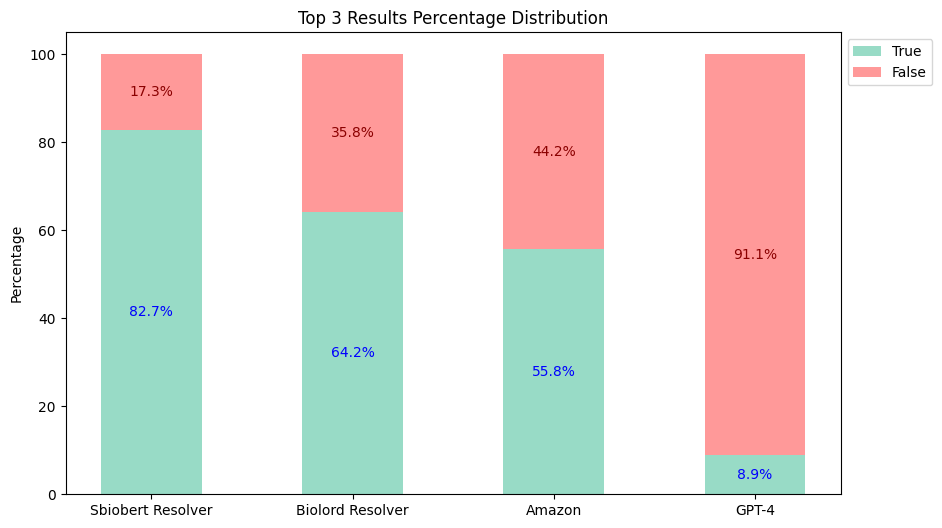
- Healthcare NLP returns up to 25 closest results, and Amazon Medical Comprehend returns up to five results, both sorted starting from the closest one. In contrast, the GPT-4 returns only one result, so its scores are reflected similarly in both charts.
- Since the performance of GPT-4 and GPT-4o is almost identical according to the official announcement, and we used both versions for the accuracy calculation. Additionally, the GPT-4 returns only one result, which means you will see the same results in both evaluation approaches.
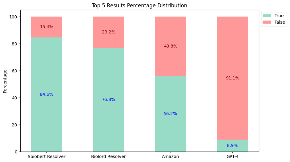
- Two approaches were adopted for evaluating these tools, given that the model outputs may not precisely match the annotations:
- Top-3: Compare the annotations to see if they appear in the first three results.
- Top-5: Compare the annotations to see if they appear in the first five results.
Accuracy Results
- Top-3 Results:
- Top-5 Results:
Price Analysis Of The Tools
Since we don’t have such a small dataset in real world, we calculated the price of these tools according to 1M clinical notes.
-
Open AI Pricing: We created a prompt to achieve better results, which costs $3.476 on GPT-4 and $1.738 GPT-4o model for the 79 documents. This means that for processing 1 million notes, the estimated cost would be $44,000 for the GPT-4 and $22,000 for the GPT-4o.
-
Amazon Comprehend Medical Pricing: According to the price calculator, obtaining RxNorm predictions for 1M documents, with an average of 9,700 characters per document, costs $24,250.
-
Healthcare NLP Pricing: When using John Snow Labs-Healthcare NLP Prepaid product on an EC2-32 CPU (c6a.8xlarge at $1,2 per hour) machine, obtaining the RxNorm codes for medications (excluding the NER stage) from approximately 80 documents takes around 2 minutes. Based on this, processing 1M documents and extracting RxNorm codes would take about 25,000 minutes (416 hours, or 18 days), costing $500 for infrastructure and $4,000 for the license (considering a 1-month license price of $7,000). Thus, the total cost for Healthcare NLP is approximately $4,500.
Conclusion
Based on the evaluation results:
- The
sbiobertresolve_rxnorm_augmentedmodel of Spark NLP for Healthcare consistently provides the most accurate results in each top_k comparison. - The
biolordresolve_rxnorm_augmentedmodel of Spark NLP for Healthcare outperforms Amazon Comprehend Medical and GPT-4 models in mapping terms to their RxNorm codes. - The GPT-4 model could only return one result, reflected similarly in both charts and has proven to be the least accurate.
If you want to process 1M documents and extract RxNorm codes for medication entities (excluding the NER stage), the total cost:
- With Healthcare NLP is about $4,500, including the infrastructure costs.
- $24,250 with Amazon Comprehend Medical
- $44,000 with the GPT-4 and $22,000 with the GPT-4o.
Therefore, Healthcare NLP is almost 5 times cheaper than its closest alternative, not to mention the accuracy differences (Top 3: Healthcare NLP 82.7% vs Amazon 55.8% vs GPT-4 8.9%).
Accuracy & Cost Table
| Top-3 Accuracy | Top-5 Accuracy | Cost | |
|---|---|---|---|
| Healthcare NLP | 82.7% | 84.6% | $4,500 |
| Amazon Comprehend Medical | 55.8% | 56.2% | $24,250 |
| GPT-4 (Turbo) | 8.9% | 8.9% | $44,000 |
| GPT-4o | 8.9% | 8.9% | $22,000 |
AWS EMR Cluster Benchmark
- Dataset: 340 Custom Clinical Texts, approx. 235 tokens per text
- Versions:
- EMR Version: ERM.6.15.0
- spark-nlp Version: v5.2.2
- spark-nlp-jsl Version : v5.2.1
- Spark Version : v3.4.1
- Instance Type:
- Primary: m4.4xlarge, 16 vCore, 64 GiB memory
- Worker : m4.4xlarge, 16 vCore, 64 GiB memory
Spark NLP Pipeline:
ner_pipeline = Pipeline(stages = [
        document_assembler,
        sentence_detector,
        tokenizer,
        word_embeddings,
        ner_jsl,
        ner_jsl_converter])

resolver_pipeline = Pipeline(stages = [
        document_assembler,
        sentence_detector,
        tokenizer,
        word_embeddings,
        ner_jsl,
        ner_jsl_converter,
        chunk2doc,
        sbert_embeddings,
        snomed_resolver])
NOTES:
ner_jsl model is used as ner model.The inference time was calculated. The timer started with model.transform(df) and ended with writing results in parquet format.
The sbiobertresolve_snomed_findings model is used as the resolver model. The inference time was calculated. The timer started with model.transform(df) and ended with writing results (snomed_code and snomed_code_definition) in parquet format and 722 entities saved.
Results Table
| Partition | NER Timing | NER and Resolver Timing |
|---|---|---|
| 4 | 24.7 seconds | 1 minutes 8.5 seconds |
| 8 | 23.6 seconds | 1 minutes 7.4 seconds |
| 16 | 22.6 seconds | 1 minutes 6.9 seconds |
| 32 | 23.2 seconds | 1 minutes 5.7 seconds |
| 64 | 22.8 seconds | 1 minutes 6.7 seconds |
| 128 | 23.7 seconds | 1 minutes 7.4 seconds |
| 256 | 23.9 seconds | 1 minutes 6.1 seconds |
| 512 | 23.8 seconds | 1 minutes 8.4 seconds |
| 1024 | 25.9 seconds | 1 minutes 10.2 seconds |
CPU NER Benchmarks
NER (BiLSTM-CNN-Char Architecture) CPU Benchmark Experiment
- Dataset: 1000 Clinical Texts from MTSamples Oncology Dataset, approx. 500 tokens per text.
- Versions:
- spark-nlp Version: v3.4.4
- spark-nlp-jsl Version: v3.5.2
- Spark Version: v3.1.2
- Spark NLP Pipeline:
  nlpPipeline = Pipeline(stages=[
        documentAssembler,
        sentenceDetector,
        tokenizer,
        embeddings_clinical,
        clinical_ner,
        ner_converter
        ])
NOTE:
- Spark NLP Pipeline output data frame (except
word_embeddingscolumn) was written as parquet format intransformbenchmarks.
| Plarform | Process | Repartition | Time |
|---|---|---|---|
| 2 CPU cores, 13 GB RAM (Google COLAB) | LP (fullAnnotate) | - | 16min 52s |
| Transform (parquet) | 10 | 4min 47s | |
| 100 | 4min 16s | ||
| 1000 | 5min 4s | ||
| 16 CPU cores, 27 GB RAM (AWS EC2 machine) | LP (fullAnnotate) | - | 14min 28s |
| Transform (parquet) | 10 | 1min 5s | |
| 100 | 1min 1s | ||
| 1000 | 1min 19s |
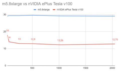
GPU vs CPU benchmark
This section includes a benchmark for MedicalNerApproach(), comparing its performance when running in m5.8xlarge CPU vs a Tesla V100 SXM2 GPU, as described in the Machine Specs section below.
Big improvements have been carried out from version 3.3.4, so please, make sure you use at least that version to fully levearge Spark NLP capabilities on GPU.
Machine specs
CPU
An AWS m5.8xlarge machine was used for the CPU benchmarking. This machine consists of 32 vCPUs and 128 GB of RAM, as you can check in the official specification webpage available here
GPU
A Tesla V100 SXM2 GPU with 32GB of memory was used to calculate the GPU benchmarking.
Versions
The benchmarking was carried out with the following Spark NLP versions:
Spark version: 3.0.2
Hadoop version: 3.2.0
SparkNLP version: 3.3.4
SparkNLP for Healthcare version: 3.3.4
Spark nodes: 1
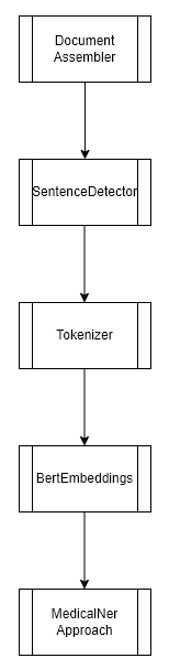
Benchmark on MedicalNerDLApproach()
This experiment consisted of training a Name Entity Recognition model (token-level), using our class NerDLApproach(), using Bert Word Embeddings and a Char-CNN-BiLSTM Neural Network. Only 1 Spark node was used for the training.
We used the Spark NLP class MedicalNer and it’s method Approach() as described in the documentation.
The pipeline looks as follows:
Dataset
The size of the dataset was small (17K), consisting of:
Training (rows): 14041
Test (rows): 3250
Training params
Different batch sizes were tested to demonstrate how GPU performance improves with bigger batches compared to CPU, for a constant number of epochs and learning rate.
Epochs: 10
Learning rate: 0.003
Batch sizes: 32, 64, 256, 512, 1024, 2048
Results
Even for this small dataset, we can observe that GPU is able to beat the CPU machine by a 62% in training time and a 68% in inference times. It’s important to mention that the batch size is very relevant when using GPU, since CPU scales much worse with bigger batch sizes than GPU.
Training times depending on batch (in minutes)
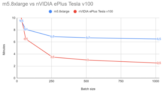
| Batch size | CPU | GPU |
|---|---|---|
| 32 | 9.5 | 10 |
| 64 | 8.1 | 6.5 |
| 256 | 6.9 | 3.5 |
| 512 | 6.7 | 3 |
| 1024 | 6.5 | 2.5 |
| 2048 | 6.5 | 2.5 |
Inference times (in minutes)
Although CPU times in inference remain more or less constant regardless the batch sizes, GPU time experiment good improvements the bigger the batch size is.
CPU times: ~29 min
| Batch size | GPU |
|---|---|
| 32 | 10 |
| 64 | 6.5 |
| 256 | 3.5 |
| 512 | 3 |
| 1024 | 2.5 |
| 2048 | 2.5 |
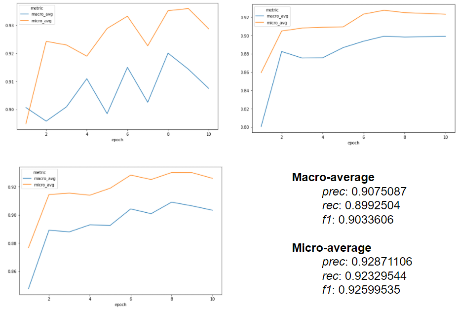
Performance metrics
A macro F1-score of about 0.92 (0.90 in micro) was achieved, with the following charts extracted from the MedicalNerApproach() logs:
Takeaways: How to get the best of the GPU
You will experiment big GPU improvements in the following cases:
- Embeddings and Transformers are used in your pipeline. Take into consideration that GPU will performance very well in Embeddings / Transformer components, but other components of your pipeline may not leverage as well GPU capabilities;
- Bigger batch sizes get the best of GPU, while CPU does not scale with bigger batch sizes;
- Bigger dataset sizes get the best of GPU, while may be a bottleneck while running in CPU and lead to performance drops;
MultiGPU Inference on Databricks
In this part, we will give you an idea on how to choose appropriate hardware specifications for Databricks. Here is a few different hardwares, their prices, as well as their performance:

Apparently, GPU hardware is the cheapest among them although it performs the best. Let’s see how overall performance looks like:

Figure above clearly shows us that GPU should be the first option of ours.
In conclusion, please find the best specifications for your use case since these benchmarks might depend on dataset size, inference batch size, quickness, pricing and so on.
Please refer to this video for further info: https://events.johnsnowlabs.com/webinar-speed-optimization-benchmarks-in-spark-nlp-3-making-the-most-of-modern-hardware?hsCtaTracking=a9bb6358-92bd-4cf3-b97c-e76cb1dfb6ef%7C4edba435-1adb-49fc-83fd-891a7506a417
MultiGPU training
Currently, we don’t support multiGPU training, meaning training 1 model in different GPUs in parallel. However, you can train different models in different GPUs.
MultiGPU inference
Spark NLP can carry out MultiGPU inference if GPUs are in different cluster nodes. For example, if you have a cluster with different GPUs, you can repartition your data to match the number of GPU nodes and then coalesce to retrieve the results back to the master node.
Currently, inference on multiple GPUs on the same machine is not supported.
Where to look for more information about Training
Please, take a look at the Spark NLP and Spark NLP for Healthcare Training sections, and feel free to reach us out in case you want to maximize the performance on your GPU.
Spark NLP vs Spacy Pandas UDF with Arrow Benchmark
This benchmarking report aims to provide a comprehensive comparison between two NLP frameworks on Spark clusters: Spark NLP and SpaCy, specifically in the context of Pandas UDF with Arrow optimization.
Spark NLP is a distributed NLP library built on top of Apache Spark, designed to handle large-scale NLP tasks efficiently. On the other hand, SpaCy is a popular NLP library in single-machine environments.
In this benchmark, we evaluate the performance of both frameworks using Pandas UDF with Arrow, a feature that enhances data transfer between Apache Arrow and Pandas DataFrames, potentially leading to significant performance gains. We will use Spacy as a UDF in Spark to compare the performance of both frameworks.
The benchmark covers a range of common NLP tasks, including Named Entity Recognition (NER) and getting Roberta sentence embeddings.
We calculated the time for both arrow enabled and disabled pandas udf for each task. We reset the notebook before each task to ensure that the results are not affected by the previous task.
Machine specs
Azure Databricks Standard_DS3_v2 machine (6 workers + 1 driver) was used for the CPU benchmarking. This machine consists of 4 CPUs and 14 GB of RAM.
Versions
The benchmarking was carried out with the following versions:
Spark version: 3.1.2
SparkNLP version: 5.1.0
spaCy version: 3.6.1
Spark nodes: 7 (1 driver, 6 workers)
Dataset
The size of the dataset is (120K), consisting of news articles that can be found here.
Benchmark on Named Entity Recognition (NER)
Named Entity Recognition (NER) is the process of identifying and classifying named entities in a text into predefined categories such as person names, organizations, locations, etc. In this benchmark, we compare the performance of Spark NLP and SpaCy in recognizing named entities in a text column.
The following pipeline shows how to recognize named entities in a text column using Spark NLP:
glove_embeddings = WordEmbeddingsModel.pretrained('glove_100d').\
    setInputCols(["document", 'token']).\
    setOutputCol("embeddings")

public_ner = NerDLModel.pretrained("ner_dl", 'en') \
    .setInputCols(["document", "token", "embeddings"]) \
    .setOutputCol("ner")

pipeline = Pipeline(stages=[document_assembler,
                              tokenizer,
                              glove_embeddings,
                              public_ner
                           ])
SpaCy uses the following pandas UDF to recognize named entities in a text column. We exclude the tagger, parser, attribute ruler, and lemmatizer components to make the comparison fair.
nlp_ner = spacy.load("en_core_web_sm", exclude=["tok2vec", "tagger", "parser", "attribute_ruler", "lemmatizer"])

# Define a UDF to  perform NER
@pandas_udf(ArrayType(StringType()))
def ner_with_spacy(text_series):
    entities_list = []
    for text in text_series:
        doc = nlp_ner(text)
        entities = [f"{ent.text}:::{ent.label_}" for ent in doc.ents]
        entities_list.append(entities)
    return pd.Series(entities_list)
Benchmark on Getting Roberta Sentence Embeddings
In this benchmark, we compare the performance of Spark NLP and SpaCy in getting Roberta sentence embeddings for a text column.
The following pipeline shows how to get Roberta embeddings for a text column using Spark NLP:
embeddings = RoBertaSentenceEmbeddings.pretrained("sent_roberta_base", "en") \
      .setInputCols("document") \
      .setOutputCol("embeddings")

pipeline= Pipeline(stages=[document_assembler,
                            embeddings
                           ])
SpaCy uses the following pandas UDF.
nlp_embeddings = spacy.load("en_core_web_trf")

# Define a UDF to get sentence embeddings
@pandas_udf(ArrayType(FloatType()))
def embeddings_with_spacy(text_series):
    embeddings_list = []
    for text in text_series:
        doc = nlp_embeddings(text)
        embeddings = doc._.trf_data.tensors[-1][0]
        embeddings_list.append(embeddings)
    return pd.Series(embeddings_list)
Results
Both frameworks were tested on a dataset of 120K rows. SpaCy was tested with and without Arrow enabled. Both frameworks utilized distributed computing to process the data in parallel.
The following table shows the time taken by each framework to perform the tasks mentioned above:
| Task | Spark NLP | Spacy UDF with Arrow | Spacy UDF without Arrow |
|---|---|---|---|
| NER extract | 3min 35sec | 4min 49sec | 5min 4sec |
| Roberta Embeddings | 22min 16sec | 29min 27sec | 29min 30sec |
Conclusions
In our analysis, we delved into the performance of two Natural Language Processing (NLP) libraries: Spark NLP and SpaCy. While Spark NLP, seamlessly integrated with Apache Spark, excels in managing extensive NLP tasks on distributed systems and large datasets, SpaCy is used particularly in single-machine environments.
The results of our evaluation highlight clear disparities in processing times across the assessed tasks. In NER extraction, Spark NLP demonstrated exceptional efficiency, completing the task in a mere 3 minutes and 35 seconds. In contrast, Spacy UDF with Arrow and Spacy UDF without Arrow took 4 minutes and 49 seconds, and 5 minutes and 4 seconds, respectively. Moving on to the generation of Roberta embeddings, Spark NLP once again proved its prowess, completing the task in 22 minutes and 16 seconds. Meanwhile, Spacy UDF with Arrow and Spacy UDF without Arrow required 29 minutes and 27 seconds, and 29 minutes and 30 seconds, respectively.
These findings unequivocally affirm Spark NLP’s superiority for NER extraction tasks, and its significant time advantage for tasks involving Roberta embeddings.
Additional Comments
- Scalability:
Spark NLP: Built on top of Apache Spark, Spark NLP is inherently scalable and distributed. It is designed to handle large-scale data processing with distributed computing resources. It is well-suited for processing vast amounts of data across multiple nodes.
SpaCy with pandas UDFs: Using SpaCy within a pandas UDF (User-Defined Function) and Arrow for efficient data transfer can bring SpaCy’s abilities into the Spark ecosystem. However, while Arrow optimizes the serialization and deserialization between JVM and Python processes, the scalability of this approach is still limited by the fact that the actual NLP processing is single-node (by SpaCy) for each partition of your Spark DataFrame.
- Performance:
Spark NLP: Since it’s natively built on top of Spark, it is optimized for distributed processing. The performance is competitive, especially when you are dealing with vast amounts of data that need distributed processing.
SpaCy with pandas UDFs: SpaCy is fast for single-node processing. The combination of SpaCy with Arrow-optimized UDFs can be performant for moderate datasets or tasks. However, you might run into bottlenecks when scaling to very large datasets unless you have a massive Spark cluster.
- Ecosystem Integration:
Spark NLP: Being a Spark-native library, Spark NLP integrates seamlessly with other Spark components, making it easier to build end-to-end data processing pipelines.
SpaCy with pandas UDFs: While the integration with Spark is possible, it’s a bit more ‘forced.’ It requires careful handling, especially if you’re trying to ensure optimal performance.
- Features & Capabilities:
Spark NLP: Offers a wide array of NLP functionalities, including some that are tailored for the healthcare domain. It’s continuously evolving and has a growing ecosystem.
SpaCy: A popular library for NLP with extensive features, optimizations, and pre-trained models. However, certain domain-specific features in Spark NLP might not have direct counterparts in SpaCy.
- Development & Maintenance:
Spark NLP: As with any distributed system, development and debugging might be more complex. You have to consider factors inherent to distributed systems.
SpaCy with pandas UDFs: Development might be more straightforward since you’re essentially working with Python functions. However, maintaining optimal performance with larger datasets and ensuring scalability can be tricky.
Small GGUF LLM Speed Benchmarks on Databricks
This benchmark measures the inference speed of small GGUF language models within Healthcare NLP on Databricks (AWS). Two model families were tested (jsl_meds_4b and jsl_meds_8b) under different quantizations (q16, q8, q4) using 100 rows of input data. Three clinical NLP tasks were evaluated: Summarization, Named Entity Recognition (NER), and Question Answering.
- Dataset: Clinical texts used for summarization, NER, and question answering tasks.
- Cluster Configuration:
- CPU Cluster: i3.4xlarge - 122 GB Memory, 16 Cores
- GPU Cluster: g4dn.xlarge [T4] - 16 GB Memory, 4 Cores
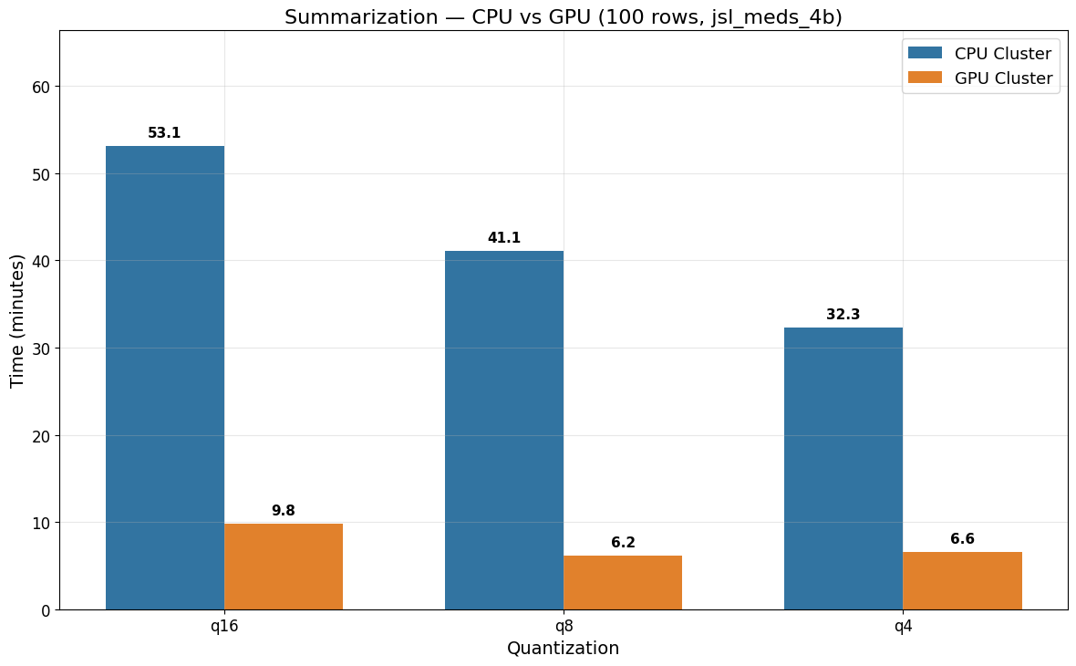
Summarization Benchmark (jsl_meds_4b)
| Model | Quantization | CPU Cluster | GPU Cluster |
|---|---|---|---|
| jsl_meds_4b_q16_v5 | q16 | 53 min 6 sec | 9 min 51 sec |
| jsl_meds_4b_q8_v5 | q8 | 41 min 8 sec | 6 min 11 sec |
| jsl_meds_4b_q4_v5 | q4 | 32 min 17 sec | 6 min 34 sec |
GPU acceleration provides up to a 6.7x speedup for the Summarization task (q8: 41 min 8 sec on CPU vs 6 min 11 sec on GPU). Lower quantization levels reduce runtimes on CPU (q16 > q8 > q4), while on GPU the differences between q8 and q4 are minimal.
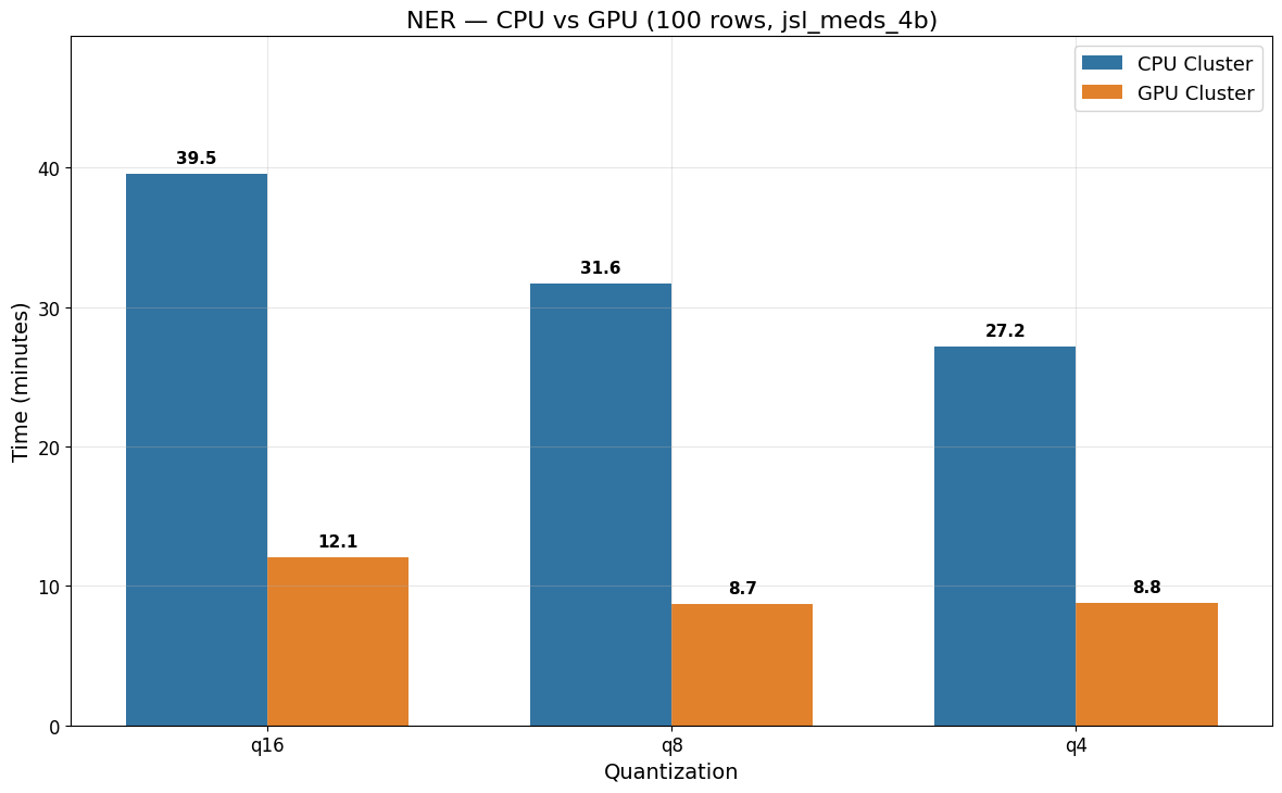
NER Benchmark (jsl_meds_4b)
| Model | Quantization | CPU Cluster | GPU Cluster |
|---|---|---|---|
| jsl_meds_4b_q16_v5 | q16 | 39 min 32 sec | 12 min 5 sec |
| jsl_meds_4b_q8_v5 | q8 | 31 min 39 sec | ~8 min 42 sec |
| jsl_meds_4b_q4_v5 | q4 | 27 min 12 sec | ~8 min 49 sec |
NER benefits from GPU acceleration, with a speedup of up to 3.6x (q8: 31 min 39 sec on CPU vs ~8 min 42 sec on GPU). Lower quantization consistently reduces CPU runtimes, while on GPU, q8 and q4 perform similarly.
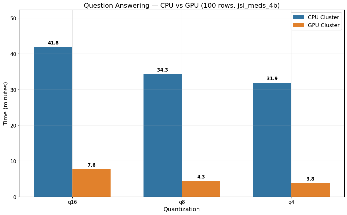
Question Answering Benchmark (jsl_meds_4b)
| Model | Quantization | CPU Cluster | GPU Cluster |
|---|---|---|---|
| jsl_meds_4b_q16_v5 | q16 | 41 min 50 sec | 7 min 37 sec |
| jsl_meds_4b_q8_v5 | q8 | 34 min 17 sec | 4 min 21 sec |
| jsl_meds_4b_q4_v5 | q4 | 31 min 52 sec | 3 min 45 sec |
Question Answering benefits strongly from GPU acceleration, achieving up to an 8.5x speedup (q4: ~32 min on CPU vs ~4 min on GPU).
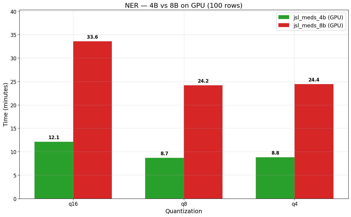
NER Benchmark (jsl_meds_8b)
| Model | Quantization | CPU Cluster | GPU Cluster |
|---|---|---|---|
| jsl_meds_8b_q16_v4 | q16 | 1 h 52 min 32 sec | 33 min 34 sec |
| jsl_meds_8b_q8_v4 | q8 | 1 h 27 min 57 sec | 24 min 12 sec |
| jsl_meds_8b_q4_v4 | q4 | 1 h 6 min 49 sec | 24 min 26 sec |
The 8B model requires longer inference times than the 4B model on both CPU and GPU. At 100 rows, GPU acceleration provides up to a 3.6x speedup for 8B (q8: 1 h 27 min 57 sec on CPU vs 24 min 12 sec on GPU). The 4B model is faster than the 8B model on GPU across all quantizations (e.g., q16 at 100 rows: 12 min 5 sec for 4B vs 33 min 34 sec for 8B).
The figure below compares GPU runtimes between the 4B and 8B models for the NER task at 100 rows:
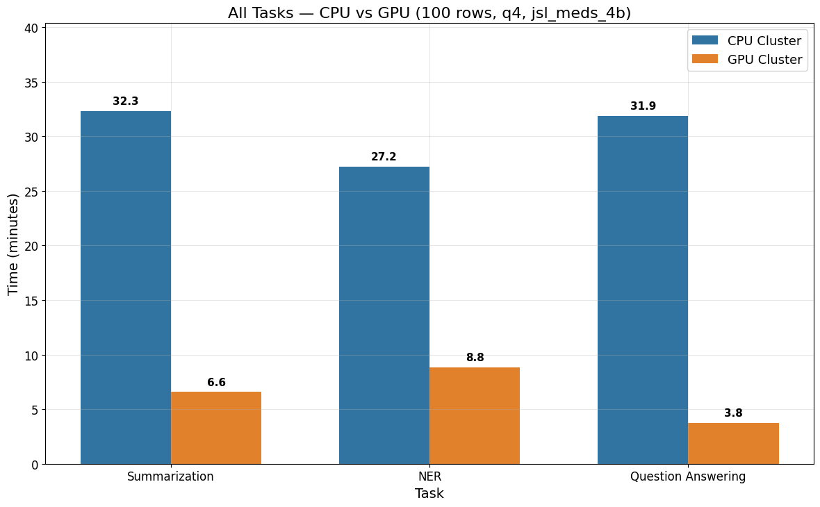
Cross-Task Comparison (100 rows, q4, jsl_meds_4b)
The figure below compares CPU and GPU runtimes across all three tasks using the q4 quantization at 100 rows. All three tasks benefit from GPU acceleration, with Question Answering showing the largest speedup (~8.5x), followed by Summarization (~4.9x) and NER (~3.1x).
Takeaways
- GPU acceleration is most impactful for Summarization and Question Answering tasks, where speedups of up to 6.7x and 8.5x were observed respectively. NER also benefits with up to 3.6x speedup;
- Quantization generally reduces inference times on CPU, where q4 is the fastest across all tasks. On GPU, q8 and q4 perform similarly for Summarization and NER;
- NER tasks benefit from GPU acceleration for both the 4B model (~3.6x speedup) and the 8B model (~3.6x speedup);
- Model size: the 8B models require noticeably longer runtimes than 4B models on both CPU and GPU. The 4B model is faster than the 8B model across all configurations; Note: Benchmark results may vary based on hardware specifications, model versions, and system configurations. These results are specific to the tested environment and should be used as a relative performance guide.